Integration#
강좌: 수치해석
Newton-Cotes#
사다리꼴 공식#
적분 구간을 사다리꼴 면적으로 계산
\[ I = \int_a^b f(x) dx \approx \int_a^b f_1(x)dx = \int_a^b \left [ f(a) + \frac{f(b) - f(a)}{b -a} (x-a) \right ] dx \]

Fig. 17 Trapezoid rule (from Wikipedia)#
오차
\[ E_t = -\frac{1}{12} f''(\xi) (b-a)^3 \]유도
Newton 보간식
\(\alpha = \frac{x-a}{h}\), \(h=b-a\), \(\Delta f(a) = f(b) - f(a)\) 일때
\[\begin{align} I &= \int_a^b \left [ f(a) + \Delta f(a)\alpha + \frac{f''(\xi)}{2} \alpha (\alpha-1)h^2 \right ] dx \end{align} \]\(f''(\xi)\) 가 거의 변하지 않는 상수로 가정하면
\[\begin{split}\begin{align} I & \approx h \left [ \alpha f(a) + \frac{\alpha^2}{2} \Delta f(a) + \left ( \frac{\alpha^3}{6} - \frac{\alpha^2}{4} \right) f''(\xi) h^2 \right ]_0^1 \\ & = h \left [ f(a) + \frac{\Delta f(a) }{2} \right ] - \frac{1}{12} f''(\xi) h^3 \\ & = h \frac{f(a) + f(b)}{2} - \frac{1}{12} f''(\xi) h^3 . \end{align} \end{split}\]
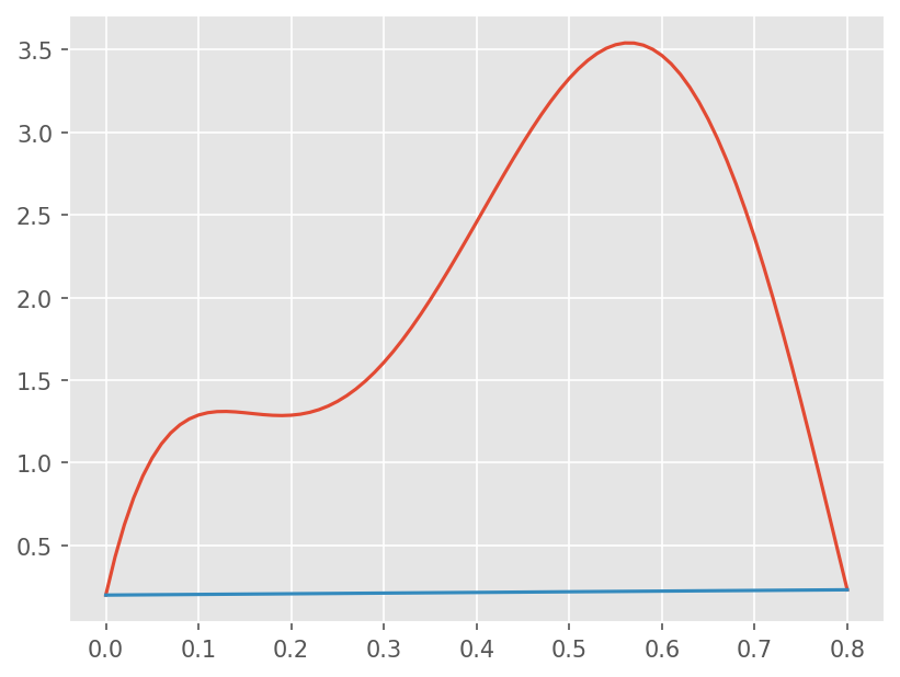
예제#
\(f(x) = 0.2 + 25x - 200 x^2 + 675x^3 -900 x^4 + 400 x^5\) 을 \([0, 0.8]\) 구간에서 적분하시오.
Exact Integration \(I_{exact} = 1.640533\)
%matplotlib inline
from matplotlib import pyplot as plt

import numpy as np

plt.style.use('ggplot')
plt.rcParams['figure.dpi'] = 150
# function
f = lambda x: 0.2 + 25*x - 200*x**2 + 675*x**3 -900*x**4 +400*x**5

# Interval
a, b = 0, 0.8

# Value at both ends
fa, fb = f(a), f(b)

# Plot
x = np.linspace(a, b, 81)

plt.plot(x, f(x))
plt.plot([a, b], [fa, fb])

# Trapezoidal rule
Itrap = 0.5*(fa + fb)*(b-a)
print(Itrap)
0.1728000000000225
다중 적분 (Composite trapezoid rule)#
\([a, b]\) 구간을 여러 간격으로 (sub intervals) 나눠서 적분

Fig. 18 Composite Trapezoid rule (from Wikipedia)#
(n+1) 개 점으로 등간격 분할
\(h = (b-a)/n\)
\[\begin{split} \begin{align} I &= \int_{x_0}^{x_1} f(x) dx + \int_{x_1}^{x_2} f(x) dx + ... + \int_{x_{n-1}}^{x_n} f(x) dx \\ & \approx h \frac{f(x_0) + f(x_1)}{2} + h \frac{f(x_1) + f(x_2)}{2} + ... + h \frac{f(x_{n-1}) + f(x_n)}{2} \\ &= \frac{h}{2} \left [ f(x_0) + 2\sum_{i=1}^{n-1} f(x_i) + f(x_n) \right ] \end{align} \end{split}\]오차
\[ E_t = \sum_{i=1}^n -\frac{1}{12} f''(\xi_i) (h)^3 = -\frac{(b-a)^3}{12n^3} \sum_{i=1}^n f''(\xi_i) \approx -\frac{(b-a)^3}{12n^2} \bar{f}'' \]예제
# function
f = lambda x: 0.2 + 25*x - 200*x**2 + 675*x**3 -900*x**4 +400*x**5
Ie = 1.640533

# Interval
a, b = 0, 0.8

# Num of sub-interval
n = 2

# Trapezoid rule
h = (b-a)/n
I = (f(a) + 2*sum([f(a + i*h) for i in range(1, n)]) + f(b))* h/2
print(I)

# Increasing n
for n in range(2, 11):
    h = (b-a)/n
    I = (f(a) + 2*sum([f(a + i*h) for i in range(1, n)]) + f(b))* h/2
    et = abs((I-Ie)/Ie)*100
    print("{}, {:.4f}, {:.4f}, {:.1f}".format(n, h, I, et))
1.0688000000000115
2, 0.4000, 1.0688, 34.9
3, 0.2667, 1.3696, 16.5
4, 0.2000, 1.4848, 9.5
5, 0.1600, 1.5399, 6.1
6, 0.1333, 1.5703, 4.3
7, 0.1143, 1.5887, 3.2
8, 0.1000, 1.6008, 2.4
9, 0.0889, 1.6091, 1.9
10, 0.0800, 1.6150, 1.6
DIY#
(Single and Composite) Trapezoid 적분 계산 함수를 구성하시오.
Simpson’s Rule#
구간 내를 다항식으로 근사해서 적분 정확도 향상
Simpson 1/3 rule#
구간 내에 3개의 등간격 점을 이용해서 2차 Lagrange 다항식으로 근사해서 적분
\[\begin{split} \begin{align} I &\approx \int_a^b f_2(x)dx \\ &= \int_a^b \left [ \frac{(x-x_1)(x-x_2)}{(x_0-x_1)(x_0-x_2)} f(x_0) +\frac{(x-x_0)(x-x_2)}{(x_1-x_0)(x_1-x_2)} f(x_1) +\frac{(x-x_0)(x-x_1)}{(x_2-x_0)(x_2-x_1)} f(x_2) \right ] dx\\ &= \frac{h}{3}[f(x_0) + 4f(x_1) + f(x_2)] = \frac{b-a}{6}[f(x_0) + 4f(x_1) + f(x_2)] \end{align} \end{split}\]\(h=(b-a)/2\)

Fig. 19 Simpson 1/3 rule (from Wikipedia)#
오차
\[ E_t = -\frac{1}{90} h^5 f^{(4)}(\xi) = - \frac{(b-a)^5}{2880} f^{(4)} (\xi) \]유도
Newton 보간식
\(\alpha = \frac{x-a}{h}\), \(h=(b-a)/2\), \(\Delta^n f(a)\) 은 제차분식
\[\begin{align} I &= \int_0^2 \left [ f(a) + \Delta f(x_0)\alpha + \frac{\Delta^2 f(x_0)}{2} \alpha (\alpha-1) + \frac{\Delta^3 f(x_0)}{6} \alpha (\alpha-1)(\alpha-2) + \frac{f^{(4)}(\xi)}{24} \alpha (\alpha-1)(\alpha-2)(\alpha-3) h^4 \right ] d \alpha \end{align} \]\(f^{(4)}(xi)\) 가 거의 변하지 않는 상수로 가정하면
\[\begin{split}\begin{align} I & \approx h \left [ \alpha f(x_0) + \frac{\alpha^2}{2} \Delta f(a) + \left ( \frac{\alpha^3}{6} - \frac{\alpha^2}{4} \right) \Delta^2 f(x_0) + \left ( \frac{\alpha^4}{24} - \frac{\alpha^3}{6} + \frac{\alpha^2}{6} \right) \Delta^3 f(x_0) + \left ( \frac{\alpha^5}{120} - \frac{\alpha^4}{16} + \frac{11\alpha^3}{72} - \frac{\alpha^2}{8} \right) f^{(4)}(\xi) h^4 \right ]_0^2 \\ & = h \left [ 2f(a) + 2\Delta f(x_0) + \frac{\Delta^2 f(x_0)}{3} + (0) \Delta^3 f(x_0) \right ] - \frac{1}{90} f^{(4)}(\xi) h^5 \\ & = \frac{h}{3} [f(x_0) + 4 f(x_1) + f(b)] - \frac{1}{90} f^{(4)}(\xi) h^5 \end{align} \end{split}\]
다중 적분 (Composite Simpson 1/3 rule)#
(n+1) 개 점으로 등간격 분할 (짝수)
\(h = (b-a)/n\)
\[\begin{split} \begin{align} I &= \int_{x_0}^{x_2} f(x) dx + \int_{x_2}^{x_4} f(x) dx + ... + \int_{x_{n-2}}^{x_n} f(x) dx \\ & \approx 2h \frac{f(x_0) + 4 f(x_1) + f(x_2)}{6} + 2h \frac{f(x_2) + 4 f(x_3) + f(x_4)}{6} + ... + 2h \frac{f(x_{n-2}) + 4 f(x_{n-1}) + f(x_n)}{6} \\ &=\frac{b-a}{3n} \left [ f (x_0) + 4 \sum_{i=1,3,5}^{n-1} f(x_i) + 2\sum_{i=2,4,6}^{n-2} f(x_i) + f(x_n) \right ] \end{align} \end{split}\]오차
\[ E_a = -\frac{(b-a)^5}{180 n^4} \bar{f}^{(4)} \]
Simpson 3/8 rule#
구간 내에 4개의 등간격 점을 이용해서 2차 Lagrange 다항식으로 근사해서 적분
\[\begin{split} \begin{align} I &\approx \int_a^b f_3(x)dx \\ &= \frac{3h}{8}[f(x_0) + 3f(x_1) + 3f(x_2) + f(x_3)] = \frac{b-a}{8}[f(x_0) + 3f(x_1) + 3f(x_2) + f(x_3)] \end{align} \end{split}\]\(h=(b-a)/3\)
오차
\[ E_t = -\frac{3}{80} h^5 f^{(4)}(\xi) = - \frac{(b-a)^5}{6480} f^{(4)} (\xi) \]다중 적분시, 홀수개 분활에 사용
예제#
앞선 문제를 Simpson rule로 풀어보시오.
Composite Simpson 1/3 rule로 풀어보시오.
# function
f = lambda x: 0.2 + 25*x - 200*x**2 + 675*x**3 -900*x**4 +400*x**5

# Interval
a, b = 0, 0.8

# Value at both ends
fa, fb = f(a), f(b)

# Simpson 1/3
def simpson13(f, a, b):
    x0, x1, x2 = a, 0.5*(a+b), b

    return (b-a)/6*(f(x0) + 4*f(x1) + f(x2))


# Simpson 3/8
def simpson38(f, a, b):
    x0, x1, x2, x3 = a, (2*a + b)/3, (a +2*b)/3, b

    return (b-a)/8*(f(x0) + 3*f(x1) + 3*f(x2) + f(x3))


I13 = simpson13(f, a, b)
print(I13)

I38 = simpson38(f, a, b)
print(I38)
1.3674666666666742
1.519170370370378
# function
f = lambda x: 0.2 + 25*x - 200*x**2 + 675*x**3 -900*x**4 +400*x**5
Ie = 1.640533

# Interval
a, b = 0, 0.8

# Sub-interval
n = 4
xi = np.linspace(a, b, n + 1)

# Composite integration
(f(xi[0]) + 4*sum(f(xj) for xj in xi[1:-1:2]) + 2*sum(f(xj) for xj in xi[2:-2:2]) + f(xi[-1]))* (b-a)/ (3*n)
1.6234666666666717
# function
f = lambda x: 0.2 + 25*x - 200*x**2 + 675*x**3 -900*x**4 +400*x**5
Ie = 1.640533

# Interval
a, b = 0, 0.8

for n in [4, 6, 8, 10]:
    xi = np.linspace(a, b, n + 1)
    I = (f(x[0]) + 4*sum(f(xj) for xj in xi[1:-1:2]) + 2*sum(f(xj) for xj in xi[2:-2:2]) + f(xi[-1]))* (b-a)/ (3*n)
    et = abs((I-Ie)/Ie)*100
    print("{}, {:.4f}, {:.1f}".format(n, I, et))
4, 1.6235, 1.0
6, 1.6372, 0.2
8, 1.6395, 0.1
10, 1.6401, 0.0
Romberg Integration#
Richardson Extrapolation#
정확도가 낮은 수치적분 기법을 활용하여 고차 수치 적분을 외삽
Trapezoid intgration을 사용하는 경우
\[ I_1 \approx \frac{h}{2} \left [ f(x_0) + 2\sum_{i=1}^{n-1} f(x_i) + f(x_n) \right ] + c_1 h^2 + c_2 h^4 + ... \]간격을 절반으로 하면
\[ I_2 \approx \frac{h}{4} \left [ f(x_0) + 2\sum_{i=1}^{n-1} f(x_i) + f(x_n) \right ] + c_1 \frac{h^2}{4} + c_2 \frac{h^4}{16} + ... \]
두 식에서 Leading error 항을 제거하기 위해
\[ I_{12} = \frac{4 I_2 - I_1}{3} = I + \frac{1}{4}c_2 h^4 + ... \]
Romberg integation#
Rihcardson extrapolation 일반화
\[ I_{j,k} = \frac{4^{k-1} I_{j+1, k-1} - I_{j,k-1}}{4^{k-l} - 1} \]
예제#
# Trapezoid rule with decreasing the size of sub-interval
I1 = []
for n in [2, 4, 8]:
    h = (b-a)/n
    I = (f(a) + 2*sum([f(a + i*h) for i in range(1, n)]) + f(b))* h/2
    et = abs((I-Ie)/Ie)*100
    print("{}, {:.4f}, {:.4f}, {:.1f}".format(n, h, I, et))
    I1.append(I)

print(I1)

# Romberg Integration
k = 2
I21 = (4**(k-1)*I1[1] -I1[0]) / (4**(k-1)-1)
I22 = (4**(k-1)*I1[2] -I1[1]) / (4**(k-1)-1)
I2 = [I21, I22]
print(I2)

# Romberg Integration
k = 3
I3 = (4**(k-1)*I2[1] -I2[0]) / (4**(k-1)-1)

print(I3)
2, 0.4000, 1.0688, 34.9
4, 0.2000, 1.4848, 9.5
8, 0.1000, 1.6008, 2.4
[1.0688000000000115, 1.4848000000000068, 1.600800000000004]
[1.623466666666672, 1.6394666666666697]
1.6405333333333363
Gauss (-Legendre) Integration#
적분 좌표와 Weighting 계수를 조절해여 고차 정확도 적분
\[ I = \int_a^b f(x) dx = \sum_i w_i f(\xi_i) \]Transformation: \(\xi=\frac{x - \frac{a+b}{2}}{\frac{b-a}{2}}\)
2 Points#
두점으로 3차 함수를 정확하게 적분하는 공식
\(f(x)=1, x, x^2, x^3\)
\[\begin{split} \begin{align} w_0 f(x_0) + w_1 f(x_1) &= \int_{-1}^1 1 dx = 2 \\ w_0 f(x_0) + w_1 f(x_1) &= \int_{-1}^1 x dx = 0 \\ w_0 f(x_0) + w_1 f(x_1) &= \int_{-1}^1 x^2 dx = \frac{2}{3} \\ w_0 f(x_0) + w_1 f(x_1) &= \int_{-1}^1 x^3 dx = 0 \end{align} \end{split}\]연립방정식의 해
\(w_0 = w_1 = 1\)
\(x_0 = -\frac{1}{\sqrt{3}}, x_1 = \frac{1}{\sqrt{3}}\)
일반 구간
\[ I = \int_a^b f(x) dx = \frac{b-a}{2} \int_{-1}^{1} f(\xi) d\xi \]
다점 Gauss-Legendre Quadrature rule#
See Wikipeida
예제#
# function
f = lambda x: 0.2 + 25*x - 200*x**2 + 675*x**3 -900*x**4 +400*x**5
Ie = 1.640533

# Interval
a, b = 0, 0.8

# Transformation [-1, 1 ] -> [a, b]
xi_to_x = lambda xi: (a+b)/2 + xi*(b-a)/2

# 2 Points rule
w0=w1 = 1
xi0, xi1 = -1/np.sqrt(3), 1/np.sqrt(3)

# Gauss Qaudrature
I = (w0*f(xi_to_x(xi0)) + w1*f(xi_to_x(xi1))) *(b-a) /2
print(I)
1.8225777777777772
# function
f = lambda x: 0.2 + 25*x - 200*x**2 + 675*x**3 -900*x**4 +400*x**5
Ie = 1.640533

# Interval
a, b = 0, 0.8

# Transformation [-1, 1 ] -> [a, b]
xi_to_x = lambda xi: (a+b)/2 + xi*(b-a)/2

# 3 points rule
xi = -np.sqrt(3/5), 0 , np.sqrt(3/5)
w = 5/9, 8/9, 5/9

# Gauss quadrature
I = 0
for wi, xii in zip(w, xi):
    I += wi*f(xi_to_x(xii))

I *= (b - a)/2
print(I)
1.6405333333333294
Scipy 활용#
Scipy 내 integrate 모둘에서 수치 적분에 대한 여러 함수를 제공한다.
수치 적분:
scipy.integrate모듈